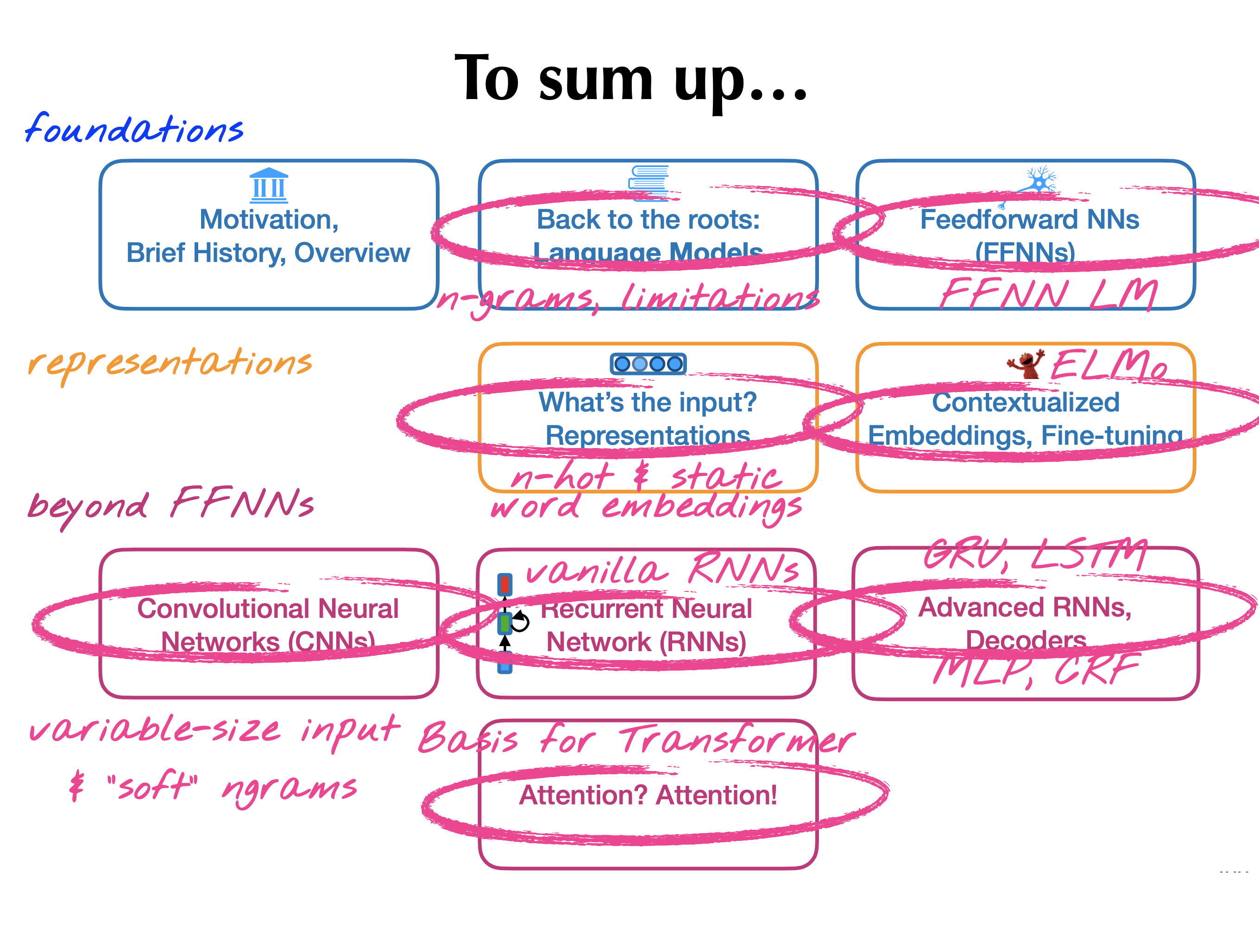
Highlights of AthNLP Summer School 2019 - Part I
This post discusses the highlights of Athens NLP Summer School 2019. The sessions covered core concepts on Language Modelling, Machine Translation, POS Tagging & Question Answering.
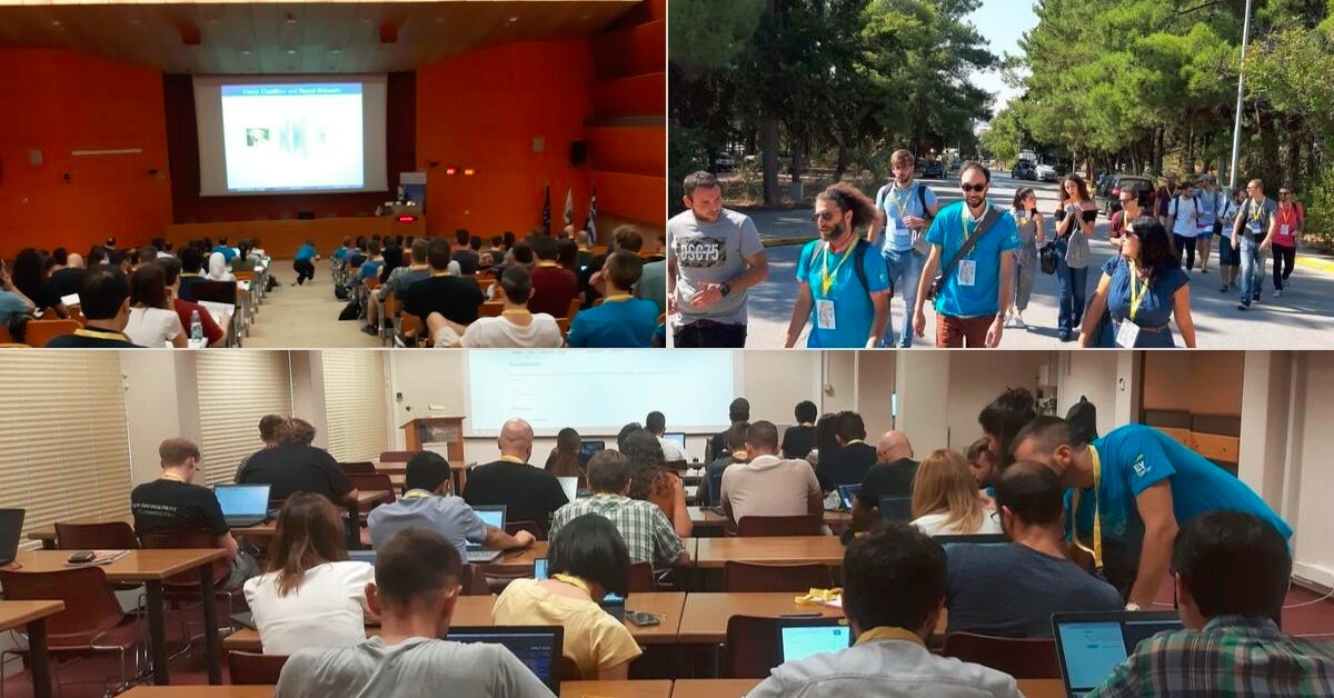
Table of Content
I had the opportunity to attend my first international summer school from 18-25th September, 2019 at National Center for Scientific Research “Demokritos”, Athens, Greece. AthNLP is an annual event where students, researchers and industry experts with interests in Language Processing, Computational Linguistics and Statistics gather to attain a deeper understanding of the domain.
The week consisted of lectures from accomplished researchers, workshops, poster sessions from participants and social events. This post summarizes the key learnings from the school assuming a basic understanding of NLP and mathematics.
The complete lecture playlist can be accessed here.
Classification in NLP [PPT]
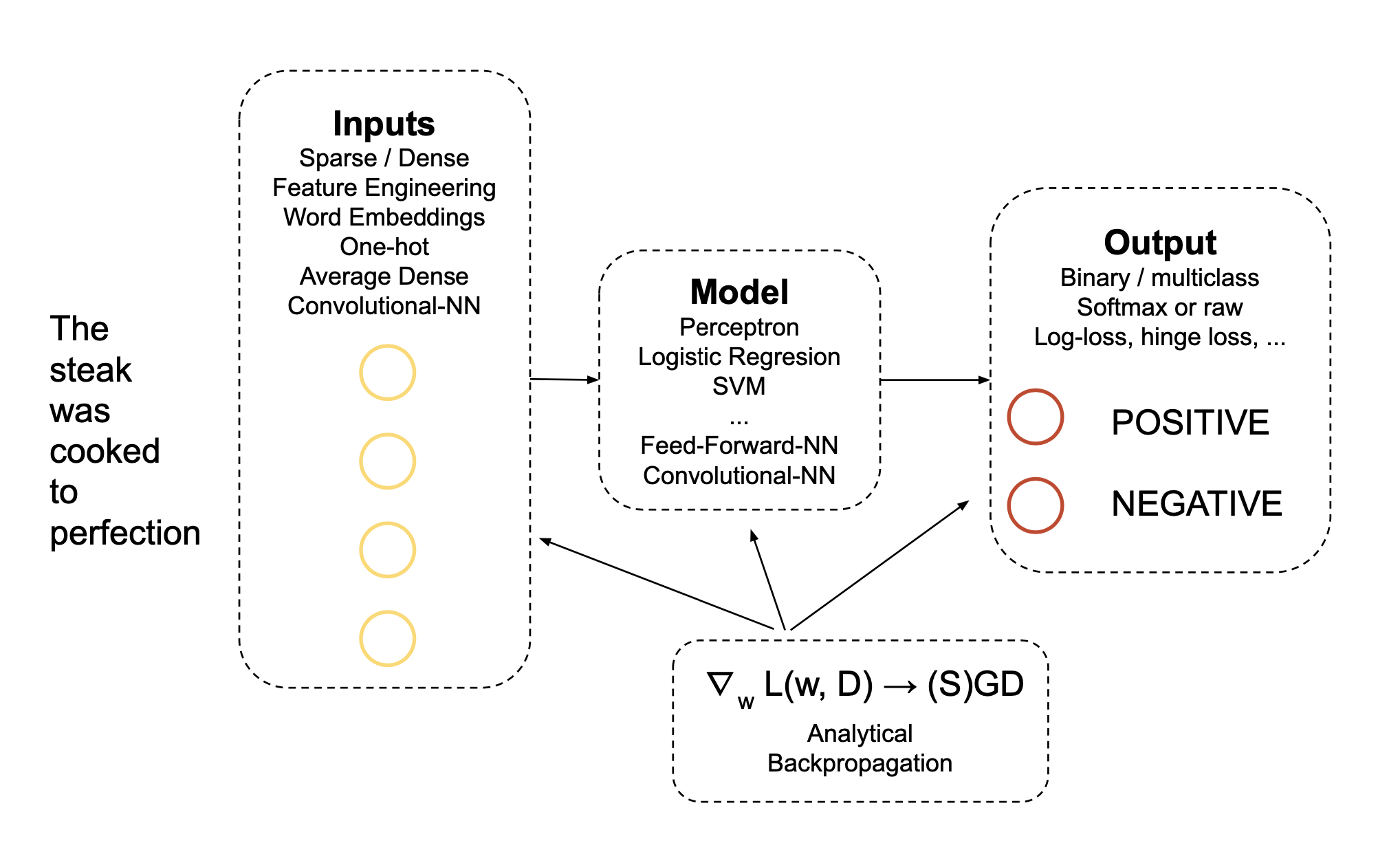
The school commenced with a session on Classification in NLP by Ryan Mcdonald from Google. Broad topics in the lecture include linear classifiers, feature representation & perceptron. Classification tasks in NLP can be mainly categorized as binary classification (eg: fact checking- fake/real) & multi-class classification (eg:topic identification).
Understanding the principles of linear classifiers (LC) are the key to understanding modern neural networks. These LC’s can be stacked together to form classical NLP pipelines where each classifier’s prediction is used to handcraft features for others classifiers. For instance in the task of sentiment classification, we could first build a LC for part-of-speech (POS) tagging as these documents contains too many adjectives (good, bad, happy) and then use these POS tags as features for our final sentiment model.
Try to answer this question to test your grasp on this topic:
What happens if we don’t use any activation function in a multilayer neural network?
Yes. The network will behave as a linear classifier !!
Formally the task of classification can be stated as: Given a labelled data with input-output (i-o) pairs ${(x_n,y_n)}_{n=1}^N \subset \mathcal{X} \times \mathcal{Y}$, the goal is to learn a classifier $h: \mathcal{X}\rightarrow\mathcal{Y}$ from the space of classifiers that generalizes well on arbitrary inputs. Instead of mapping only the input, we map the i-o pairs to a sparse-binary feature representation. Score for a specific label is obtained using linear combination of features and weights (model parameter).
\[\hat{y}= h(x)= \text{argmax} \sum\limits_i w_i \phi(x,y)_i\]The only distinction between various LC’s (perceptron, SVM, Logistic Regression) is the way in which this parameter $w$ is learned. The set of feature representations remain the same but the strategies used to learn parameters for those features are different.
Structured Prediction in NLP [PPT]
After looking at the binary and multi-class classification, Xavier Carreras from dMetrics introduced another type of classification known as Structured Prediction. Consider the task of Named Entity Recognition (NER) for instance. It might appear that it’s a multi-class classification task as the goal is to predict a label for each word in a sequence. But if we follow this approach then “London” would result in the output “Location” in the following sentence.
| Jack | London | went | to | Paris |
|---|---|---|---|---|
| PER | PER | - | - | LOC |
Instead we can make use of the surrounding inputs and their outputs. If the next word is went, it is highly unlikely that a “location” can go somewhere. Also, it is more probable that if the previous word is a “Person” then “London” is also a person rather than a “Location”.
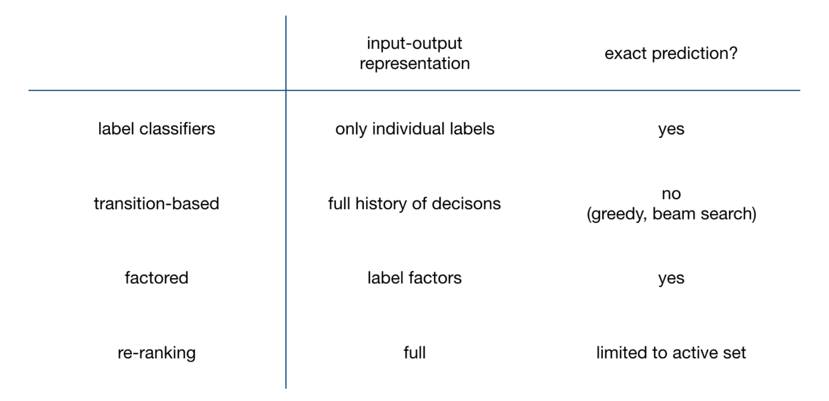
In general, structured prediction methods can be classified as:
- Label Classifiers
- Transition based systems
- Factor models
- Re-Ranking
Label Classifiers
Instead of considering surrounding sequence, we consider this as a multi-class classification task over individual labels $l$ for each input position $t$. As we already discussed above this is the simplest approach but does not allow us to capture interaction between output labels.
\[\hat{y}_t = \underset{l \in \{LOC, PER, -\}}{\text{argmax}} \text{score}(x,t,l)\]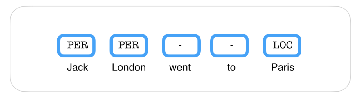
Transition-based Sequence Prediction
Overcoming the drawback of previous method, in transition based models, we not only have the token of current position and candidate label but also the previous predictions.
\[\hat{y}_t = \underset{l \in \{LOC, PER, -\}}{\text{argmax}} \text{score}(x,t,l, \hat{y}_{1:t-1})\]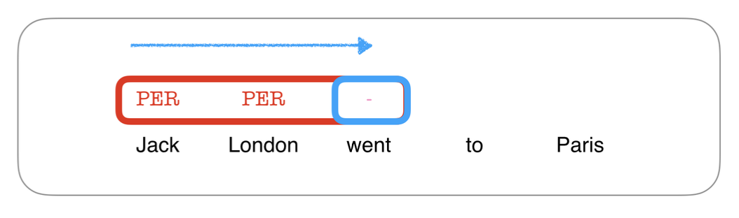
Factored Sequence Prediction
Influenced from the above two approaches, this approach predicts the complete output sequence at once by introducing a factor for each input word which is the current label and the previous label. This is an intermediate approach as we are performing a multi-class classification (label classifiers) for each input word but with the help of both current and previous label rather than the full sequence of previous decisions (transition-based).
\[\hat{y} = \underset{y \in y_n}{\text{argmax}}\sum\limits_{i=1}^n \text{score}(x,i,y_{i-1},y_i)\]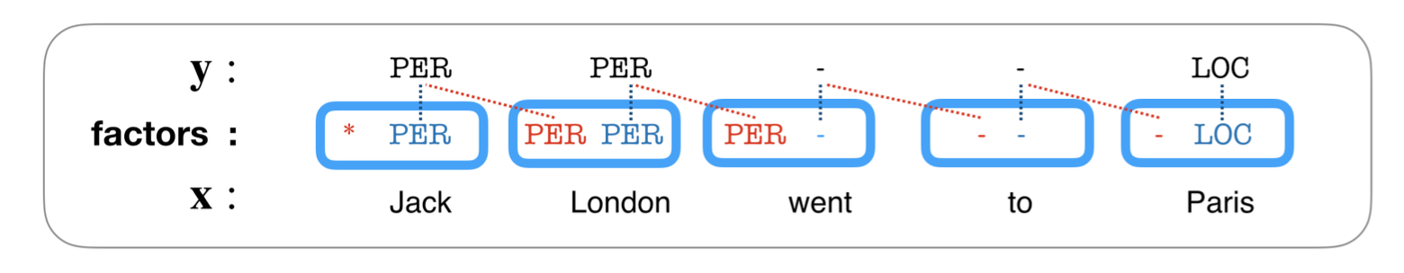
Re-Ranking
Re-Ranking approach makes use of the full input sequence and all the possible output sequences. A base model (can be any previous model) is used to first rank all the sequences in some way and then select most likely output sequences referred as an active set. This active set can give the full representation by looking at any input and output making it fully expressive.
\[\hat{y} = \underset{y \in A(y_n)}{\text{argmax}} \quad\text{score}(x,y)\]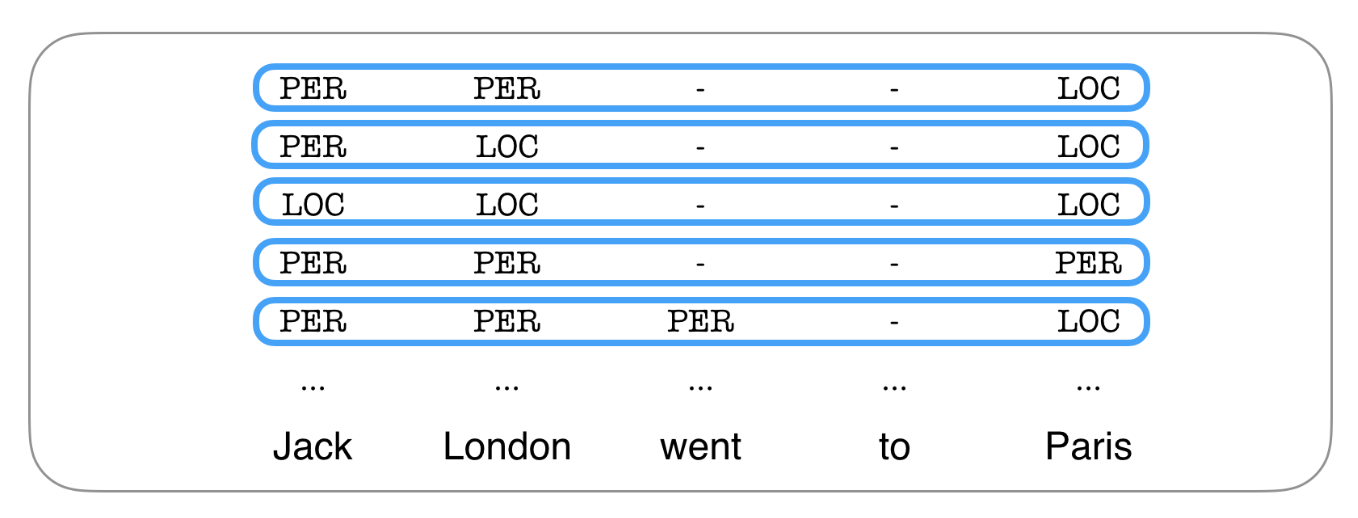
Summary of Structured Prediction Approaches
Encoder-Decoder Neural Nets [PPT]
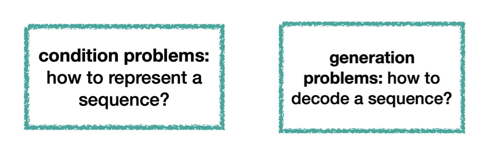
Barbara Plank kicked off the third day with one of the most interesting session on Sequential Models. So far we only discussed conditioning on sequential data to make a classification i.e Condition problems. But applications like auto-complete and spelling correction require us to generate sequential data instead of classifying it i.e. Generation Problems.
This gives rise to Language Models (LMs) which can be used to compute either the probability of a text or probability of next word given some text. Earlier approaches used chain rule to estimate the joint probability of the entire sequence by multiplying conditional probabilities of some word given previous words. This was based on the $n^{th}$ order Markov assumption that the probability of a current word only depends only upon the previous $n$ words, hence the name $n$-gram language models. However, these n-gram LMs have difficulty handling long-range dependencies due to the problem of sparsity with increasing $n$ and also in sharing strength among similar words.
Similar words issue was handled by fixed-window based neural LM which iteratively moved the n-gram window through a very large corpus to predict the next word by concatenating the embeddings of words in current window at each time step.
Consequently, Recurrent Neural Networks (and their variants) became one of the promising architectures which can not only handle long-term dependencies by eliminating the markov assumption but can also handle arbitrary length inputs like CNNs.